Denormalization vs Normalization for Analytical Query Performance

Denormalization vs normalization for analytical query performance depends on how the engine reads data. In columnar systems, column pruning and predicate pushdown make denormalization a structural default. The useful decision is how far to take it, given the queries, update costs, and people or agents that will use the data.

Why columnar engines treat joins differently from row-oriented databases

A row-oriented engine stores each row contiguously, so reading a column means reading the row around it. Under that arrangement, narrow tables limit the data brought into a scan, and joining them can be cheaper than scanning a wide table full of repeated attributes. Width has a direct reading cost.

A columnar engine changes the relationship by storing each column’s values sequentially in its own blocks. Reading three columns from a hundred-column table means reading only the blocks for those three columns. A join, however, still requires the engine to reconstruct relationships between separate tables. With a columnar engine, the row-store tradeoff changes because keeping repeated data out can add query-time work while saving little scan I/O.

How column pruning and predicate pushdown make wide tables cheaper, not more expensive

Column pruning is the first mechanism behind that difference. The engine reads only the columns the query needs, including those named in its SELECT and WHERE clauses. A wider table is not automatically a more expensive table to query.

Predicate pushdown also helps by moving filters toward the storage layer, before the data goes into memory for more processing. Where those filters can eliminate irrelevant row groups, the engine avoids decoding them. Co-location makes this more useful. When the attributes needed for filtering and aggregation live together, the engine can apply the filters within a single scan rather than assemble the relevant attributes through joins.

Consider a query that counts events for users with a particular attribute. In a normalized schema, the events table supplies the events, while the users table supplies the attribute and the relationship needed to select matching users. The engine must read from both and resolve that relationship. With the user attribute embedded in a wide events table, the query filters and counts from the same table, reading only the needed columns. Its other embedded user attributes remain unread.

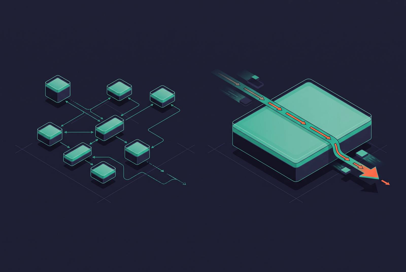
Could the normalized query filter the users table first? It can, but that does not remove the work of matching users to events. Pushdown within a table is not the same as eliminating a join across tables. Denormalization removes that boundary from the query path. Its advantage comes from letting pruning and filtering work together on co-located data.

Why denormalization is the assumed data model for columnar analytical engines, not an optimization applied after the fact

Analytical workloads often scan many rows but read only a few columns. Columnar storage is built for that pattern, and wide tables provide it directly. The engine can process batches of thousands of values within a column rather than reconstruct each business relationship before answering the query. Joins interrupt that simple scan path. Even when an engine executes joins efficiently, it must do work that a prejoined representation has already moved out of query time.

The star schema makes this design principle concrete without requiring every attribute to sit in one table. It collapses dimension attributes from many normalized source tables into a small number of wide dimension tables around a central fact table. This is already deliberate partial denormalization. It reduces join depth while retaining separation for large, slowly changing dimensions. Its role as a canonical analytical schema shows that denormalization is part of the starting design.

The one big table pattern takes the same principle further by embedding dimension attributes directly in the fact table. That removes the remaining dimension joins from queries against it. The choice is architectural rather than cosmetic. This works well when dimensions stay the same, queries are complex, and the engine gains a lot from single-pass scans. Viewed this way, denormalization pre-computes joins, exchanging storage and write complexity for less work on each read.

Where denormalization creates real costs, and what the Star Schema Benchmark evidence shows

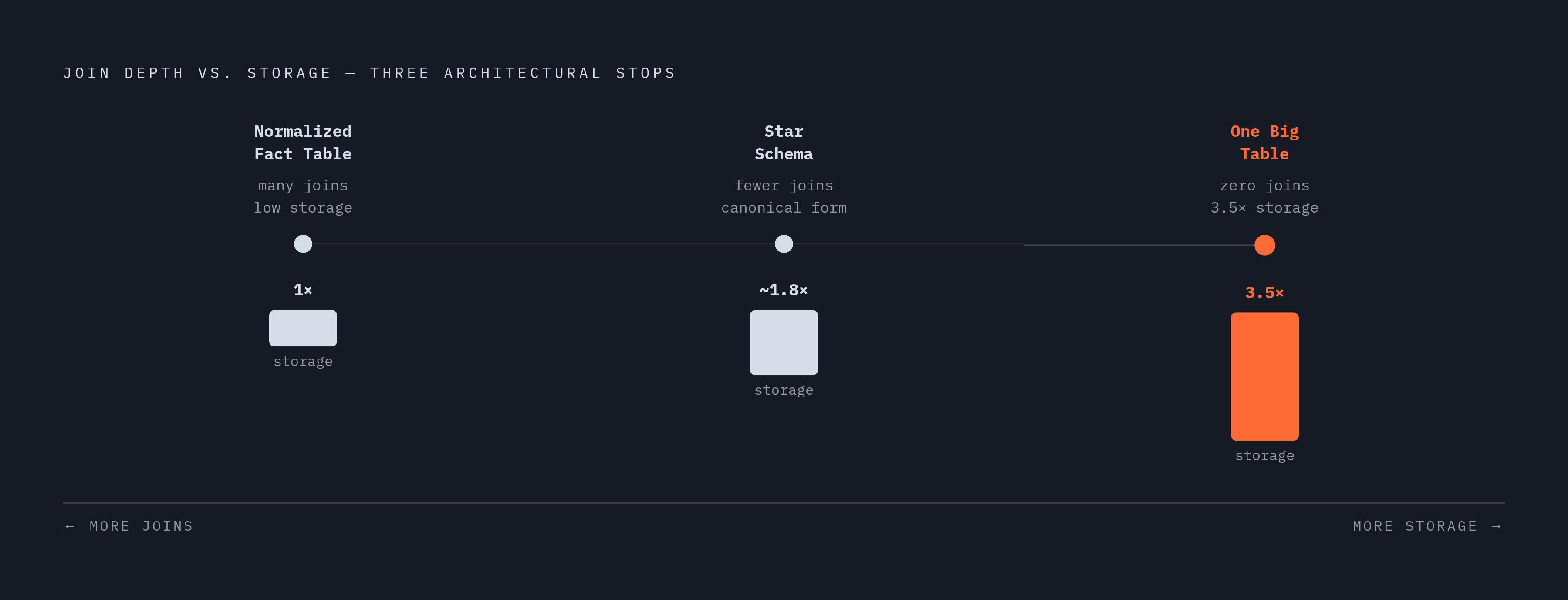
Pre-computing those relationships means storing their results over and over, so faster reads come with storage amplification. A fully flat table stores the same dimension attributes in every fact row they apply to. That can make its footprint substantially larger than the normalized fact table. Pruning does not erase that storage bill. Nor does it guarantee that every query against the larger representation will outperform a query joining a fact table to a small dimension.

Research using the Star Schema Benchmark found that solutions “performed very differently depending on the schema.” The benchmark evidence includes a fully denormalized flat table roughly three-and-a-half times larger than the normalized fact table alone at scale. For narrow query patterns, the larger footprint can become a liability even with fewer joins. The evidence challenges a universal performance promise.

A query that routinely combines many dimensions can avoid substantial reconstruction work when those attributes are embedded. A query that needs only one small dimension has less join work to remove. Its balance can favor the star schema. Column pruning keeps unrelated columns out of the scan, but the benchmark shows why that mechanism alone is not a complete prediction of execution time.

Updates still have a cost, even when reads are faster. If a denormalized copy must reflect a customer name change or product category reassignment, every fact row containing that attribute needs to remain consistent with the source. A separate dimension can record the change in one row. Repetition therefore multiplies maintenance work as well as storage. Full denormalization is most compelling when its avoided joins justify both costs.

A practical decision framework for where to draw the normalization boundary in an analytical schema

The practical question for a schema designer is where to separate normalized source layers from denormalized serving layers. Source and staging layers need a canonical representation in which writes preserve integrity and avoid update anomalies. Third normal form is a good fit for that role. The analytical layer has a different job, because reads dominate and repeated joins can become the bottleneck. The serving model should be chosen for those reads.

Within that serving layer, the first test is how many dimensions the dominant queries combine. If queries routinely cross many dimensions, full embedding gives pruning and pushdown the strongest opportunity to operate over co-located attributes. If the main queries touch only one or two dimensions, a star schema may offer a better balance. The number of tables alone says little about how much useful join work a change would save.

The next test is whether the attributes are stable enough to replicate cheaply. Attributes that stay the same or change slowly need less update work than those whose denormalized copies must be corrected often. A defined update path is essential here. The operational guidance is to denormalize one column at a time, with an explicit way to keep its copy consistent with the source. That discipline separates deliberate denormalization from a schema that merely accumulated duplicate data.

Mixed workloads also create a reason to stop short of flattening the base tables. A materialized view can pre-compute joins for high-traffic query paths while leaving the underlying schema normalized. Frequent queries use the view, while rare queries use the base tables. This preserves a useful boundary between workloads. Consumer clarity is another test, because a serving schema must also be understandable to the people and agents choosing which attributes to query.

How AI agents querying schemas change the denormalization calculus further

AI agents may need to do database work to learn the schema before they start an analytical query. An agent using a tool such as Model Context Protocol may inspect table names, column names, data types, keys, and constraints before generating SQL. A person writing the query may already know those relationships. The agent has to discover them first. That turns the number and complexity of tables into an additional source of latency and compute use.

A normalized schema asks the agent to traverse more relationships and may require more exploratory queries before it can assemble an answer. A few wide tables give the agent less to explore because related attributes are together. Fewer relationships need to be inferred or explored. After discovery, the generated query benefits from the same column pruning and predicate pushdown available to a human-written query.

This is not a guarantee of better generated SQL for every task. Ryosuke Kohita’s study, “Exploring Database Normalization Effects on SQL Generation,” found that denormalized schemas helped simple retrieval, while normalized schemas performed better for aggregation queries affected by duplication and NULL values. The study also found that examples could reduce difficulties with normalized schemas. Correctness remains a separate test from speed. An easy-to-discover table still has to support the intended aggregation without misleading the query generator.

Agent workloads can also issue many queries rapidly and in parallel, exploring the same data from different angles. Per-query join overhead then accumulates faster than in human-paced analysis. Accountability adds another design concern. Wide schemas with full query logging make analytical intent easier to reconstruct, while numerous possible join paths can produce more varied SQL for the same goal. Isolated, read-only compute over shared denormalized data, with every query logged, addresses both performance and accountable access without treating schema shape as the whole solution.

What the remaining objection — smarter optimizers closing the gap — actually proves

The strongest objection is that better optimizers can make normalized analytical schemas cheaper to query. The cited benchmarks show gains of 25 to 45 percent for AI-enhanced query planners on complex analytical workloads that use normalized structures. If join reconstruction becomes cheap enough, the storage and consistency costs of embedding attributes may no longer be justified for a particular workload. A decision based on an older join penalty can become the wrong decision.

But reducing a cost is not eliminating it. Better planners change when pre-computing a join pays off, but the tradeoff remains. Vectorized join engines also make queries run better, though the tables stay separate and their attributes are still not co-located. The comparison still involves the whole system. A hybrid HTAP system can outperform a dedicated OLAP solution in mean execution time for certain workloads, showing why schema design cannot be judged apart from engine architecture.

The lesson for engineers is to benchmark actual query patterns with the schema alternatives their update requirements can support. An optimizer can compensate for join-heavy design, but relying on that compensation without examining the storage path leaves an important choice unexamined. Optimizer quality belongs in the decision. The goal is to understand why columnar engines favor denormalization well enough to choose its boundary deliberately and independently of the source database.